Demand Forecasting with Azure Machine Learning (AML)

This article helps you to understand the components of Demand Forecasting with Azure Machine Learning (AML).

CONTENT   Introduction Demand Forecasting Demand Forecasting Parameters Considerations to Avoid Flat Forecasting

INTRODUCTION

Dynamics 365 Supply Chain Management provides the end-to-end planning capabilities that manufacturers, distributors, and retailers require to meet their supply chain needs. Functionality ranges from demand forecasting, demand planning, master planning, and order processing. 

The focus of this article is Demand Forecasting. 

Let’s get started.

DEMAND FORECASTING

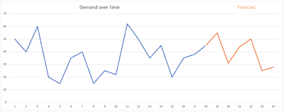
Demand forecasting is to predict future demand for products and services. This information is required to estimate revenue and drive strategic and operational business planning. Benefits include reducing cost by minimizing the buffer on-hand inventory, reducing lead times by ordering long lead time items ahead of time, increasing revenue for providing availability, and helping strategic business decisions on global capacity planning with data-driven knowledge.

The ultimate Purpose is to provide time to plan resources, plant expansion, capital equipment purchase, and anything requiring a long lead time to purchase.

The logic is to Gather transactional historical data and use machine learning to generate anticipated (expected) demand with Azure Machine Learning.

After the demand is created, forecast planning is run to calculate gross requirements for materials and capacity, and to generate planned orders.

Demand Patterns

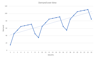
When historical data for demand are plotted against a time scale, they will show shapes or consistent patterns. A pattern is the general shape of a time series that shows the actual demand varies from period to period.

Dynamics 365 Supply Chain Management generates time series forecasting by using Azure Machine Learning. Time series forecasting refers to models that use previous demand values to predict future demand. Time series forecasting is affected by 3 elements (Demand Patterns): Trend, seasonality, and variation.

Trend: General direction in which demand is moving. The longer the window, the smoother the trend will be.

Seasonality: In time series data, seasonality, is the presence of variations that occur at specific regular intervals, which refers to periodic fluctuations. For example, electricity consumption is high during the day and low during the night, or online sales increase during Christmas before slowing down again.

Variation: Unexplained or random variation in the time series. This will be discussed in tracking the forecast.

By using the 3 elements above, different forecasting tools use different statistical forecasting algorithms in different ways and predict demand.

Dynamics 365 Supply Chain Management and Azure Machine Learning allow businesses to compare different forecasting models and select the best predicting demand.

Mathematical Formula Components

An automated time-series experiment is treated as a multivariate regression problem. Past time-series values are "pivoted" to become additional dimensions for the regressor together with other predictors. This approach, unlike classical time series methods, has the advantage of naturally incorporating multiple contextual variables and their relationship to one another during training. Automated ML learns a single, but often internally branched model for all items in the dataset and prediction horizons. More data is thus available to estimate model parameters and generalization to unseen series becomes possible.

A subset of data is used to train the forecasting model, and it’s possible to specify what type of model validation to perform. Automated ML performs model validation as part of training. That is, automated ML uses validation data to tune model hyperparameters based on the applied algorithm to find the combination that best fits the training data. 

D365 parameters are forecasting settings and are used to make decisions on how to use the dataset and predict demand. 

Forecast accuracy is represented with MAPE (Mean Absolute Percentage Error), the estimated accuracy of the forecasting model that is used to generate the predictions.

MAPE compares the actual vs forecasted value and gives the distance of how close the forecasted values are to actual demand. A good forecast’s maximum MAPE value is 20.

You can view the accuracy percentage under Model details - MAPE on the Demand forecast details page

DEMAND FORECASTING PARAMETERS

General: All items must have a unit conversion setup that relates to the demand forecasting unit.

Select which types of transactions should be included in the historical data.

Select forecast generation strategy Azure Machine Learning vs Copy over historical demand. Before version 10.0.24, the forecast generation strategy for Azure was the Azure Machine Learning Classic which is a service that’s going to be deprecated.

Forecast dimensions: In addition to company, site, and allocation key, it is possible to include more information as the forecast dimension.

Each row of the generated forecast is a unique combination of the enabled values aka granularity attribute. The forecast will be running for each granularity attribute that is based on forecast dimensions.

Item allocation keys: Item allocation keys are groups of items used to generate a forecast together and allow the system to improve the performance of forecast generation (Similar to batch threading where different allocation keys are in parallel to generate a forecast). Additionally, transaction types can be chosen along with different forecast algorithm parameters for each item allocation key. An item must be a part of an item allocation key in order to be included in the forecast generation process.

Outliner removal: It’s a standalone parameter. Outliner removal helps to exclude outliers (exceptional data or extreme values) from the historical data that is used to calculate a demand forecast. Master planning > Setup > Demand forecasting > Outlier removal. 

Reduce forecast requirements: It’s a master plan parameter. When the master plan is run, planned orders are generated based on the forecast. But the forecast needs to be adjusted when real sales orders (actual demand) start coming for the forecasted period. Forecast reduction keys are used for that purpose. If a reduction key is not used, the forecast requirements aren't reduced during master scheduling. In this case, master planning creates planned orders to supply the forecasted demand (forecast requirements). These planned orders maintain the suggested quantity, regardless of other types of demand. For example, if sales orders are placed, master planning creates additional planned orders to supply the sales orders. The quantity of the forecast requirements isn't reduced. Master planning > Setup > Plans > Master plans > General fast tab.

Forecast algorithm parameters are used by Azure and R (a language and environment for statistical computing and graphics) to create the forecast model. The R package forecast provides methods and tools for displaying and analyzing univariate time series forecasts including exponential smoothing via state space models and automatic ARIMA modeling.

Time series models: ARIMA, ETS, STL, ETS + ARIMA, ETS + STL, and ALL. When ALL is used, the system runs through all of the models and picks the model that has the lowest MAPE value. Use this model if there is no data scientist available to see what model is chosen and to analyze the data. This model consumes more time than others, in other words, has the worst performance.

Minimum and Maximum forecasted value: Forced minimum or maximum forecast values. The system doesn’t generate any forecast when the estimated forecast value is ZERO instead, this parameter value is used. On the other side, the allowed maximum value can be limited, as well.

Missing value substitution: This is about what happens when there is a gap in the historical data. Missing value can be replaced with a number or average of previous and following data or previous value or linear or polynomial interpolation. The most common use is to use ZERO since there may not be real data or demand on that date.

Missing value substitution scope: This is about what happens when there is a gap in the historical data. Substitution rule can be applied to the whole history, or to a specific granularity attribute. The advised value is to apply the substitution to all of the data.

Confidence level: It is the range of possible future demand values that the system generates.

Seasonality hint: It is the number of seasonal patterns that data scientist think of. For example; if data has a quarterly seasonality pattern, and forecasting is in monthly buckets, the Seasonality value should be 3.

Force seasonality: For the models using seasonality, it is possible to specify what the relationship between trend and seasonality is.

The test set size percentage: It is the data set percentage for the testing accuracy of the forecast vs how much should be used to generate the forecast.

In general, the forecast model needs to have enough data to generate a good forecast.

CONSIDERATIONS TO AVOID FLAT FORECASTING

Test, test, and retest: Use different parameters and compare the forecast results and MAPE to arrive at the best configuration for YOUR specific data.

Involve a data scientist: Helps business to dive into the detailed areas of configuration and keeps business from getting stuck with a flat forecast.

Use R package parameters: Dynamics 365 parameters are not the full set of parameters, there are more in the R forecast package. If the results with basic configurations are not working well enough, the next step should be to review the additional parameters in the R package that cannot be changed through Dynamics 365 interface.

Use correct parameters: Correct parameters including both D365 and R need to be used to get a good MAPE measurement.

Have enough size data: Enough data needs to be used to get a good MAPE measurement. Data history needs to be twice the forecast horizon.

The ultimate purpose is to predict demand with the least error. Errors cannot be eliminated unless you are able to see to the future. The fact is as below!